by Yutaro Yamada

Around the middle of June, this paper came up: Learning to learn by gradient descent by gradient descent. For someone who’s interested in optimization and neural networks, I think this paper is particularly interesting. The main idea is to use neural networks to tune the learning rate for gradient descent.

Summary of the paper

Usually, when we want to design learning algorithms for an arbitrary problem, we first analyze the problem, and use the insight from the problem to design learning algorithms. This paper takes a one-level-above approach to algorithm design by considering a class of optimization problems, instead of focusing on one particular optimization problem.

The question is how to learn an optimization algorithm that works on a “class” of optimization problems. The answer is by parameterizing the optimizer. This way, we effectively cast algorithm design as a learning problem, in which we want to learn the parameters of our optimizer (, which we call the optimizee parameters.)

But how do we model the optimizer? We use Recurrent Neural Network. Therefore, the parameters of the optimizer are just the parameters of RNN. The parameters of the original function in question (i.e. the cost function of “one instance” of a problem that is drawn from a class of optimization problems) are referred as “optimizee parameters”, and are updated using the output of our optimizer, just as we update parameters using the gradient in SGD. The final optimizee parameters $\theta^*$ will be a function of the optimizer parameters and the function in question. In summary:

$\theta_{t+1} = \theta_t + g_t(\nabla f(\theta_t), \phi) \text{: the update equation of the optimizee parameters}$ where $g_t$ is modeled by RNN. So $\phi$is the parameter of RNN. Because LSTM is better than vanilla RNN in general (citation needed*), the paper uses LSTM. Regular gradient descent algorithms use $g_t(\nabla f(\theta_t), \phi) = -\alpha \nabla f(\theta_t)$.

RNN is a function of the current hidden state $h_t$, the current gradient $\nabla f(\theta_t)$, and the current parameter $\phi$.

The “goodness” of our optimizer can be measured by the expected loss over the distribution of a function $f$, which is

(I’m ignoring $w_t$ in the above expression of $L(\phi)$ because in the paper they set $w_t = 1$.)

For example, suppose we have a function like $f(\theta) = a \theta^2 + b\theta + c$. If $a,b,c$ are drawn from the Gaussian distribution with some fixed value of $\mu$ and $\sigma$, the distribution of the function $f$ can be defined. (Here, the class of optimization problem is a function where $a,b,c$ are drawn from Gaussian.) In this example, the optimizee parameter is $\theta$. The optimizer (i.e. RNN) will be trained by optimizing functions which are randomly drawn from the function distribution, and we want to find the best parameter $\theta$. If we want to know how good our optimizer is, we can just take the expected value of $f$ to evaluate the goodness, and use gradient descent to optimize this $L(\phi)$.

After understanding the above basics, all that is left is some implementation/architecture details for computational efficiency and learning capability.

(By the way, there is a typo in page 3 under Equation 3; $\nabla_{\theta} h(\theta)$ should be $\nabla_{\theta} f(\theta)$. Otherwise it doesn’t make sense.)

Coordinatewise LSTM optimizer

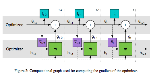
The Figure is from the paper : Figure 2 on page 4

To make the learning problem computationally tractable, we update the optimizee parameters $\theta$ coordinate-wise, much like other successful optimization methods such as Adam, RMSprop, and AdaGrad.

To this end, we create $n$ LSTM cells, where $n$ is the number of dimensions of the parameter of the objective function. We setup the architecture so that the parameters for LSTM cells are shared, but each has a different hidden state. This can be achieved by the code below:

lstm = tf.nn.rnn_cell.BasicLSTMCell(hidden_size)
for i in range(number_of_coordinates):
    cell_list[i] = tf.nn.rnn_cell.MultiRNNCell([lstm_cell] * num_layers) # num_layers = 2 according to the paper.

Information sharing between coordinates

The coordinate-wise architecture above treats each dimension independently, which ignore the effect of the correlations between coordinates. To address this issue, the paper introduces more sophisticated methods. The following two models allow different LSTM cells to communicate each other.

1. Global averaging cells: a subset of cells are used to take the average and outputs that value for each cell.
2. NTM-BFGS optimizer: More sophisticated version of 1., with the external memory that is shared between coordinates.

Implementation Notes

Quadratic function (3.1 in the paper)

Let’s say the objective funtion is $f(\theta) = \lVert W \theta - y \rVert^2$, where the elements of $W$ and $y$ are drawn from the Gaussian distribution.

$g$ (as in $\theta_{t+1} = \theta_t + g$) has to be the same size as the parameter size. So, it will be something like:

g, state = lstm(input_t, hidden_state) # here, input_t is the gradient of a hidden state at time t w.r.t. the hidden

And the update equation will be:

param = param + g

The objective function is:

The loss $L(\phi)$ can be computed by double-for loop. For each loop, a different function is randomly sampled from a distribution of $f$. Then, $\theta_t$ will be computed by the above update equation. So, overall, what we need to implement is the two-layer coordinate-wise LSTM cell. The actual implementation is here.

Results

I compared the result with SGD, but SGD tends to work better than our optimizer for now. Need more improvements on the optimization…