Spring 2015 Preview
Hey there, data lovers! Good news: Yale Data Science is back in a big way. We’ve revamped our approach for this semester and can’t wait to get going. Here’s a preview of one of our new focuses: data science vignettes. This post will take you from a question to a cool result, with some data scraping, modeling, and visualization along the way. Added bonus: you can gain insight like this quickly! This took only a couple hours of development. Data science!
As always, email us if you have questions!
Code
Introduction
Ever taken a course that you REALLY REALLY want other people to take? Ever been a professor who hasn’t been happy with your course’s enrollment and can pay a bunch of students to write reviews? Well listen up.
There has been a lot of effort put into using numerical ratings to improve our understanding of Yale’s courses. However, the review comments - which provide the richest information - have flown under the radar. For a course with high ratings, it’s probably obvious that words like “good” and “recommend” will come up frequently. Similarly, for a course with a high workload, we’d expect to see terms like “hard” and “no sleep”.
But what do highly shopped courses look like? This is the most interesting question, since the actual action someone will take after looking at reviews is to add it to their OCS worksheet (or not). By the end of this post, you’ll know what stuff to write to get people to sign up on OCS. If you aren’t interested in the methods, just skip on down to the results.
Disclaimer
Yale’s course catalog has generated quite a bit of data controversy over the year. We don’t want to add to that. We won’t display evaluations of individual courses or professors in ways that the University did not intend. If the names of any individuals or courses came up during the course of our analysis, they have been censored. We won’t host any of Yale’s data in our Github repo in accordance with University policy, but we can tell you how to get it yourselves. And we will. Right now.
The Dataset
For a given course, we’re interested in the relationship between two data sources: the content of its text reviews and the number of people who have added it to their OCS worksheet. We need to pull both of these from the web.
Text Reviews
Peter Xu and Harry Yu of CourseTable developed a crawler to read data from OCS. It’s simple to use (note: you must be a Yale student to do so). It pulls down data as a SQLite database. You can extract the course evaluation table as a comma-separated value file either from the command line or using a tool like SQLite Export.
Course Demand
Yale has recently made an effort to up its data presentation game when it comes to Shopping Period. Most notably, they constantly update demand figures on this site. We developed the Python script ocs_demand.py to extract the required data. It makes heavy use of the BeautifulSoup package to deconstruct HTML source code. On a Unix machine, use the following command to get what you want:
python ocs_demand.py | sort | uniq > ocs_demand.tsv
(Note: there’s some weird stuff going on with the course name field that we aren’t sure how to fix. We can work around it pretty easily.)
Bringing It Together
We will make the following assumption: people view all of the reviews for a course as a giant blob of text, and not individual tidbits. This seems reasonable to us, since people generally scroll through them quickly. This assumption also simplifies inference, so if you disagree with it and want to put in some extra work, that’s great.
So what we want now is a table with one row per course and the following columns: course identifier (a string), OCS demand (an integer), and the concatenated review text (a string). The Python program data_aggregate.py will handle this. As input, it takes two CSVs extracted from the CourseTable crawler - one with review data and one with course name data - and the TSV from the OCS demand script. Its design is as follows:
- Create a dictionary mapping course IDs to their concatenated review text. The review text is treated for natural language processing purposes via tokenizing, lowercasing, stopwording, and stemming. More on this later.
- Create a dictionary mapping full course names (e.g. STAT 365) to their course IDs (e.g. 17). Note that many different course names may be mapped to the same ID.
- Create a dictionary mapping course IDs to their OCS demand. This is where the dictionary from step 2 comes into play: the demand figures are associated with course names at first, and we need them associated with course IDs.
- Combine the dictionaries from steps 1 and 3 to output the desired table.
To run it on my machine, I used the following command:
python data_aggregate.py ~/workspace/enroll/data/ocs_comments.csv ~/workspace/enroll/data/course_names.csv ~/workspace/enroll/data/ocs_demand.csv ~/workspace/enroll/data/enroll_data.csv --stop --wstem
Again, we can’t provide you with data. See if you can get this to work on your own.
The Model
Let’s recap. Our goal is to see what review content will generate demand for the course on OCS. We have a table giving an ID, the demand, and the review text for every course. A simple approach would be to see which words show up frequently when the demand is high. The more sophisticated approach is to use a topic model.
Topic models comprise an important subject in machine learning, natural language processing, and graphical modeling. Essentially, a topic model is a statistical method used to identify latent clusters of elements within a collection. If you have a collection of documents composed of text, a topic model might be used to identify groupings of words, otherwise known as a topic. Every topic model relies on co-occurence; words that frequently occur together in documents are presumably of the same topic.
Perhaps the best known topic model is latent Dirichlet allocation - frequently referred to as LDA - which was introduced in 2003 by several big names: David Blei, Andrew Ng, and Michael (I.) Jordan. LDA is one of those algorithms that looks like magic when you first see it in application, and then still looks like magic after you study it. Here are some resources that can explain LDA better than we can, and we encourage you to read them.
As with many unsupervised algorithms, LDA is frequently used as a form of feature engineering. That is, it takes in “raw” data and returns something more insightful for input into a different model. This prompted David Blei and John McAuliffe to develop supervised latent Dirichlet allocation, or sLDA. By jointly modeling a response variable associated with each document, we can ensure that the topic distribution of a given document will correlate well with its response. Their example had to do with movie reviews and the star ratings associated with them. LDA might pull out topics relating to genre, but by jointly modeling the star ratings, sLDA will identify topics relating to film quality.
Implementation
Earlier, we mentioned that we somehow preprocessed the data for modeling. Here’s the motivation. Suppose the words “recommend” and “Recommending” show up in two different documents. Shouldn’t we treat them as the same object? What if the word “and” shows up? Do we even care about that? What about punctuation?
All of these cases are taken care of. Words are separated from one another by whitespace and punctuation, which is then discarded. We also discard words found on a list of common, unmeaningful English words. Words are then lowercased and weakly stemmed (meaning trailing -ing’s, -s’s, and -e’s are removed). The LDA authors themselves suggest only weakly stemming words, rather than using aggresive stemmers like the Porter algorithm.
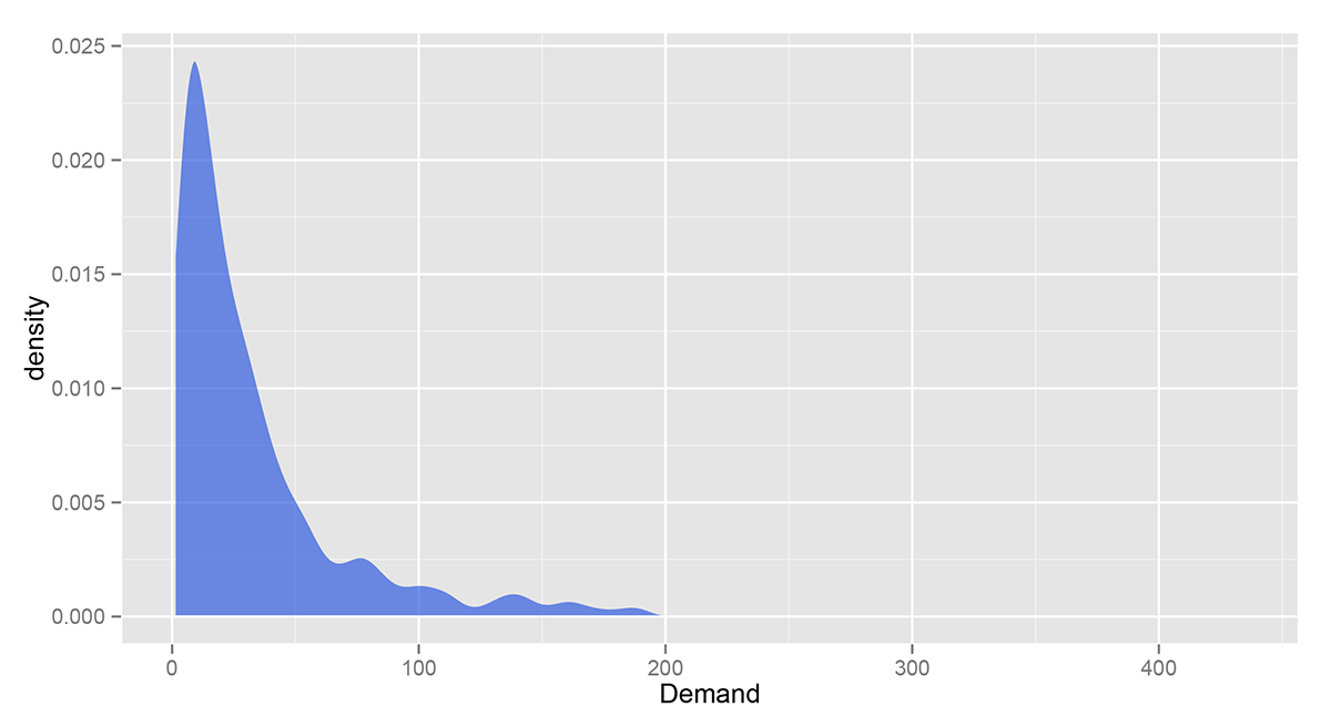
One last step of preprocessing: we’re only going to consider courses whose demand is above 50. Check out the following Gaussian kernel density estimate of the distribution of course demand. Yale offers a lot of small courses which aren’t geared towards large crowds. We aren’t interested in these.
To do the modeling, we’re going to work in R. The main script is enroll.R; note that you’ll need to modify the file paths. The lda package implements sLDA quickly and is endorsed by David Blei. It also comes with tools for text processing, namely the lexicalize function.
LDA and sLDA are bag-of-word models, meaning we only care about a word’s membership to a document, not its place within it. We can, however, recover some of the minute structure of the text by expanding our definition of a “word” from a unigram to an n-gram, or a sequence of n words found in the document. We’ll be using unigrams, bigrams, and trigrams (as implied here).
The lexicalize function only supports unigram dictionaries and document-term matrices, so we modified it in nlexicalize.R. It requires RWeka and rjava, which are sometimes difficult to deal with; if those won’t work for you, then just use the standard unigram implementation.
Picking the right parameters for your topic model can seem like more art than science, particularly choosing the number of topics. In fact, that may be the case for any model with an informative prior. With LDA, we only have some approximate measures to do model comparison (e.g. perplexity). However, the supervised version has an obvious objective metric: response prediction performance. First, we partition a training set and a test set. To identify the “best” model, we’ll use a grid search. For every parameter set in the grid, we learn an sLDA model on the training set, predict the response on the test set, and compute the RMSE. Using cross-validation or a tighter grid would give better results, but they’d also take wayyyyy too long. We’re impatient.
We can visualize the model’s performance under different parameter sets by inspecting the plot produced by the script. Here’s an example:
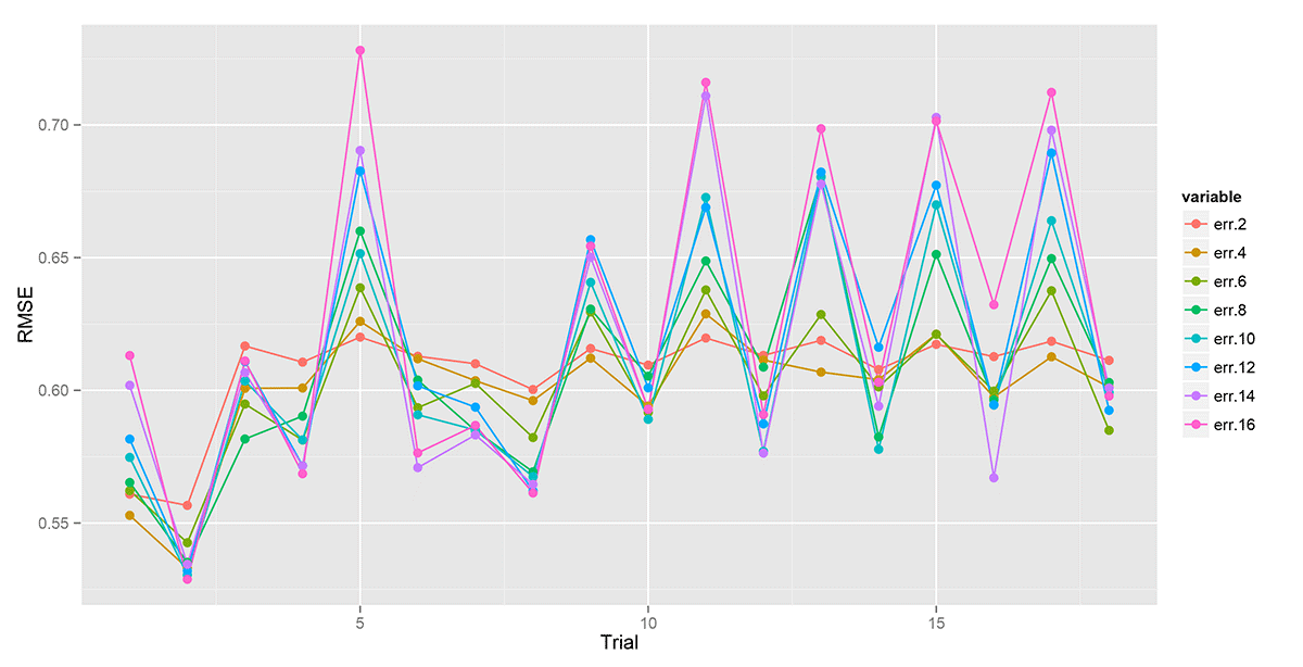
Ah! That’s confusing. Not really. Each color represents a different number of topics, and each point represents the RMSE for a different trial (i.e. parameter set). It looks like a 12 topic model always performs well, and the best Dirichlet priors are 10 for document/topic smoothing and 1 for topic/term smoothing.
We then train a final model using those values, and here’s what we found.
Results
Back to the original question: what can you write in a review to get people to sign up for a course on OCS? More specifically: what kind of language or topics separate a course attracting a decent crowd from one that attracts 400 people?
We present our results by analyzing each topic and assessing their effect on a course’s OCS demand. The latter is straightforward: in the linear model, every topic has a coefficient which represents its effect on the response. Say topic X has a large coefficient. Then a course whose reviews are highly weighted on topic X will be expected to have a large demand. Since sLDA is non-deterministic, these coefficients vary from trial to trial. However, we have found that in a 12 topic model, typically four topics strongly affect enrollment negatively and four topics strongly affect enrollment positively.
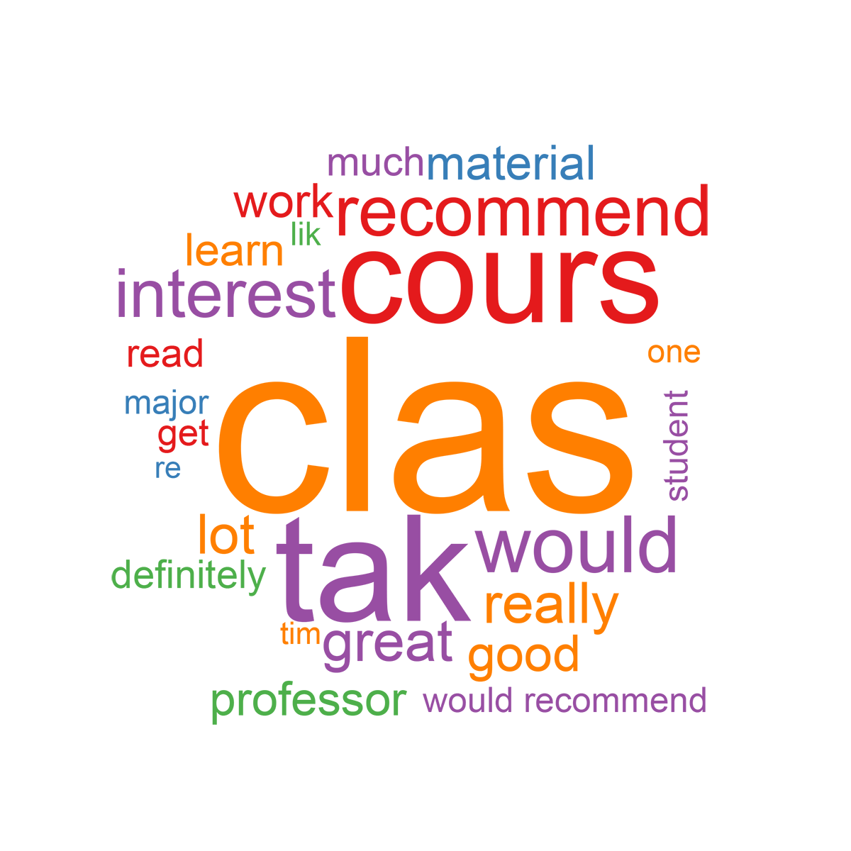
If you read up on LDA, you’ll recall that a topic is represented by a probability distribution over every term found in the collection of documents. A topic can be represented simply by the highest weighted terms in the distribution. Word clouds essentially capture the same information, but in a much more visually appealing way. The R package wordcloud is a simple way to generate world clouds directly from the results of LDA or sLDA. Due to the appearance of names of professors and courses in most of the word clouds, we will only include one example below. However, enroll.R generates all of them for your final model.
Recall that LDA and sLDA are non-deterministic, and thus the topics change from trial to trial. However, the general content of the topics are generally stable. Most notably, the most positive topic is always the one represented by the word cloud below. No surprises here. (Note: the terms have not been unstemmed, so they might be missing an s, an ing, or an e at the end.)
Next, we present a list of terms given high weights in topics that strongly effect course demand. Specifically, they are within the top 25 scoring terms in the four strongly negative or three strongly positive topics (leaving out the one presented above). Once again, they have been censored for names of professors and courses. Terms were also manually unstemmed and stopwords were added where it was obvious.
| High scoring terms; positive topics | High scoring terms; negative topics |
|---|---|
| improve | required a lot |
| grade | midterm final |
| proud | if you’re willing |
| enjoyed lecture | great however |
| take class probably | readings are long |
| manageable workload | course interesting |
| gut | clear and helpful |
| amazing class | really interesting subject |
| aquired | blend |
| low stress | highly recommend class |
| would highly recommend | incredibly |
| not much work | lecture disorganized |
| provide good background | section |
| acquired | always good |
| hard to know | use in the future |
| one paper | make or break |
| grain of salt | need qr take |
| knowledge | sense of accomplishment |
Similar terms show up on both sides, which is likely due to the fact that they occured very frequently throughout the entire corpus of reviews. So take that with a “grain of salt”. Also note that words like “terrible” aren’t showing up. Recall that we only took courses with over 50 people signed up, implying that they’re already popular.
Ok so let’s draw some conclusions. We’d expect to see many of these terms. Intuition tells us that people like courses which are high quality (“amazing class”, “enjoyed lecture”) and not-too-hard (“manageable workload”, “low stress”). Similarly, people don’t like low quality (“lecture disorganized”) or overly difficult (“required a lot”, “readings are long”) courses.
For those who say there are no guts at Yale, you may want to check the data (“gut”, “not much work”). Perhaps Yale guts aren’t as gutty as other schools’ guts. But a gut is a gut, any way you gut it.
There are also some surprises. It seems like even if people are adamant about how rewarding a class is (“clear and helpful”, “really interesting subject”, “use in future”, “sense of accomplishment”), people won’t take it. On the other hand, people seem to take some courses even if the reviewers are hesitant about it (“hard to know”, “grain of salt”).
Want to draw some more conclusions? Try running our code for yourself!
What’s Next?
The results section here just scraped the surface of what you can find from this model. For example, try adjusting the Dirichlet priors or adding topics. A model with 25 topics and smoothing priors around 0.1 or 0.01 will give topics related to individual courses.
If you want to go further, there’s always more to be done. Here are some ideas.
- Data scraping: do something similar for the course descriptions provided by professors
- Speed: create a better algorithm to match OCS demand with review text
- Debugging: what (probably ineffectual) mistake was made in the n-gram procedure and how can it be fixed?
- Modeling: construct a model using each individual review as a separate document
- Modeling (harder): jointly model individual reviews for a course and the course’s overall demand
- Visualization: generate word clouds using unstemmed words
See you at the next Yale Data Science meeting!
♥ YDS